Gradient_Descent

수치미분¶

In [6]:

def numerical_diff(f,x):
  h = 1e-4 #0.0001 
  return (f(x+h) - f(x-h)) / (2*h) # 이부분을 채워주세요! 

In [7]:

def function_1(x):
  return 0.01*x**2 + 0.1*x

In [12]:

def tangent_line(f,x):
  d = numerical_diff(f,x)
  print(d)
  y = f(x) - d*x    # 이부분을 채워주세요! 
  return lambda t: d*t + y

In [13]:

import numpy as np
import matplotlib.pylab as plt
x = np.arange(0.0, 20.0, 0.1)
y = function_1(x)
plt.xlabel("x")
plt.ylabel("f(x)")

tf = tangent_line(function_1, 5)
y2 = tf(x)

plt.plot(x,y)
plt.plot(x,y2)
plt.show()

0.1999999999990898

경사하강법(Gradient descent)¶

볼록함수(Convex Function)¶

• 어떤 지점에서 시작하더라도 최적값(손실함수가 최소로하는 점)에 도달할 수 있음

• 1-D Convex Function
  _{출처: https://www.researchgate.net/figure/A-strictly-convex-function_fig5_313821095}

• 2-D Convex Function
  
  _{출처: https://www.researchgate.net/figure/Sphere-function-D-2_fig8_275069197}

비볼록함수(Non-Convex Function)¶

• 비볼록 함수는 시작점 위치에 따라 다른 최적값에 도달할 수 있음.

• 1-D Non-Convex Function

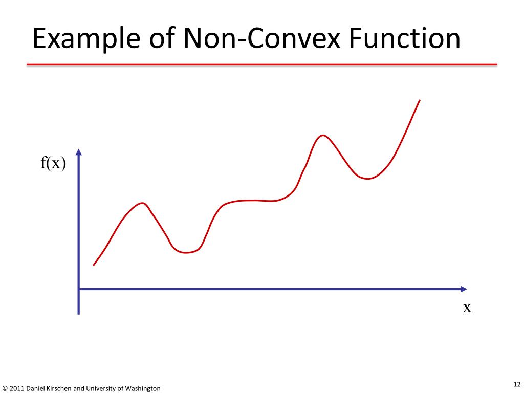
_{출처: https://www.slideserve.com/betha/local-and-global-optima}

• 2-D Non-Convex Function

_{출처: https://commons.wikimedia.org/wiki/File:Non-Convex_Objective_Function.gif}

경사하강법¶

미분과 기울기¶

• 스칼라를 벡터로 미분한 것

$\quad \frac{df(x)}{dx} = \lim_{\triangle x \to 0} \frac{f(x+\triangle x) - f(x)}{\triangle x}$¶

_{출처: https://ko.wikipedia.org/wiki/%EA%B8%B0%EC%9A%B8%EA%B8%B0_(%EB%B2%A1%ED%84%B0)}

$\quad \triangledown f(x) = \left( \frac{\partial f}{\partial x_1}, \frac{\partial f}{\partial x_2},\ ... \ , \frac{\partial f}{\partial x_N} \right)$¶

• 변화가 있는 지점에서는 미분값이 존재하고, 변화가 없는 지점은 미분값이 0
• 미분값이 클수록 변화량이 크다는 의미

경사하강법의 과정¶

• 경사하강법은 한 스텝마다의 미분값에 따라 이동하는 방향을 결정

• $f(x)$의 값이 변하지 않을 때까지 반복

  ## $\qquad x_n = x_{n-1} - \eta \frac{\partial f}{\partial x}$

  • $\eta$ : 학습률(learning rate)

• 즉, 미분값이 0인 지점을 찾는 방법

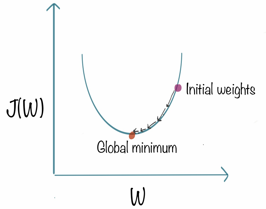
_{출처: https://www.kdnuggets.com/2018/06/intuitive-introduction-gradient-descent.html}

• 2-D 경사하강법

_{출처: https://gfycat.com/ko/angryinconsequentialdiplodocus}

경사하강법 구현¶

$\quad f_1(x) = x^2$

In [15]:

# 손실함수 정의
def f1(x):
  return x**2 # 이부분을 채워주세요!

# 손실함수를 미분한 값을 반환하는 함수 정의
def df_dx1(x):
  return 2*x # 이부분을 채워주세요!

gradient_descent 함수정의¶

매개변수로 만들어야할 5개¶

• f : 손실함수
• df_dx : 손실함수를 미분한 값을 반환하는 함수
• init_x : 초기값
• learning_rate : 학습률, 하이퍼파라미터
• step_num : 반복 횟수

In [17]:

def gradient_descent(f, df_dx, init_x, learning_rate=0.01, step_num=100):
  x = init_x
  x_log, y_log = [x], [f(x)]

  for i in range(step_num):
    grad = df_dx(x)
    x -= learning_rate * grad # 이부분을 채워주세요!

    x_log.append(x)
    y_log.append(f(x))        # x,y 값의 변화를 로그로 저장

  return x_log, y_log

경사하강법 시각화¶

In [18]:

import matplotlib.pyplot as plt
import numpy as np
plt.style.use('seaborn-whitegrid')

x_init = 5
x_log, y_log = gradient_descent(f1, df_dx1, init_x=x_init) # 이부분을 채워주세요! # 위에서 정의한 f1과 df_dx1 을 매개변수로 사용하면 됩니다.
plt.scatter(x_log, y_log, color='red')

x = np.arange(-5, 5, 0.01)
plt.plot(x, f1(x))
plt.grid()
plt.show()

학습률(learning rate)¶

• 학습률 값은 적절히 지정해야 한다!
• 너무 크면 발산하고, 너무 작으면 학습이 잘 되지 않는다.

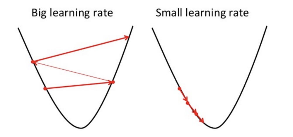_{출처: https://mc.ai/an-introduction-to-gradient-descent-algorithm/}